Kip Jordan

A statistical analysis conducted as part of the Data Science Graduate Certificate at RMIT University, Melbourne, Australia

Winter Season Analysis

Analysis of the synthetic trial data revealed that individuals in the placebo group demonstrated a 69% probability of avoiding flu infection during the winter season. This translates to approximately seven out of ten unvaccinated individuals remaining flu-free throughout the period.

Statistical analysis produced a 95% confidence interval of 59.94% to 78.06% for the proportion of unvaccinated individuals avoiding flu infection. This indicates that, with 95% confidence, the true proportion of unvaccinated individuals who will avoid flu infection falls within this range. If the trial were repeated multiple times, we would expect the proportion of uninfected individuals to fall within this interval 95% of the time.

When modelling population-wide outcomes with a 40% vaccination rate, the analysis predicts approximately 22% of the wider population would contract the flu during the season. This projection accounts for the observed infection rates in both vaccinated and unvaccinated cohorts, providing an estimate for overall population outcomes.

For individuals maintaining consistent vaccination over a decade, the analysis indicates a 7.02% probability of contracting the flu three or more times during this period. This suggests that consistently vaccinated individuals face relatively low odds (approximately 7 in 100) of experiencing three or more flu infections over ten years.

Section 1: Flu Jab Efficacy Ahead of the Winter Season

The synthetic data analysis revealed that individuals who received the placebo demonstrated a 69% probability of avoiding flu infection during the winter season. This translated to approximately seven out of ten unvaccinated individuals remaining flu-free throughout the period.

Statistical analysis produced a 95% confidence interval of 59.94% to 78.06% for the proportion of unvaccinated individuals avoiding flu infection. This indicated that, with 95% confidence, the true proportion of unvaccinated individuals who would avoid flu infection fell within this range. If the trial were repeated multiple times, we would expect the proportion of uninfected individuals to fall within this interval 95% of the time.

When modelling population-wide outcomes with a 40% vaccination rate, the analysis predicted approximately 22% of the wider population would contract the flu during the season. This projection accounted for the observed infection rates in both vaccinated and unvaccinated cohorts, providing an estimate for overall population outcomes.

For individuals maintaining consistent vaccination over a decade, the analysis indicated a 7.02% probability of contracting the flu three or more times during this period. This suggested that consistently vaccinated individuals faced relatively low odds (approximately 7 in 100) of experiencing three or more flu infections over ten years.

Section 1 Summary and Clarification

The estimated probabilities and confidence intervals provide insight into the effectiveness of the vaccine versus placebo. Given the results, we conclude that the vaccine significantly reduces the likelihood of contracting the flu. These results are meaningful for healthcare decision-makers, as the effectiveness of the vaccine can guide future health campaigns.

Section 1: Analysis Results

Outcome	Vaccinated Group	Placebo Group
Contracted flu	20	31
Remained flu-free	80	69
TOTAL	100	100

The analysis revealed that 69% of participants in the placebo group remained flu-free during the trial period.

Statistical analysis established a 95% confidence interval of 59.94% to 78.06% for flu-free participants in the placebo group.

Modelling suggested 22% of the broader population would likely contract flu during the season.

For consistently vaccinated individuals over a decade, the probability of contracting flu three or more times was 7.02%.

Section 2

Section 2: Distribution of the Sample Mean for an Exponential Distribution

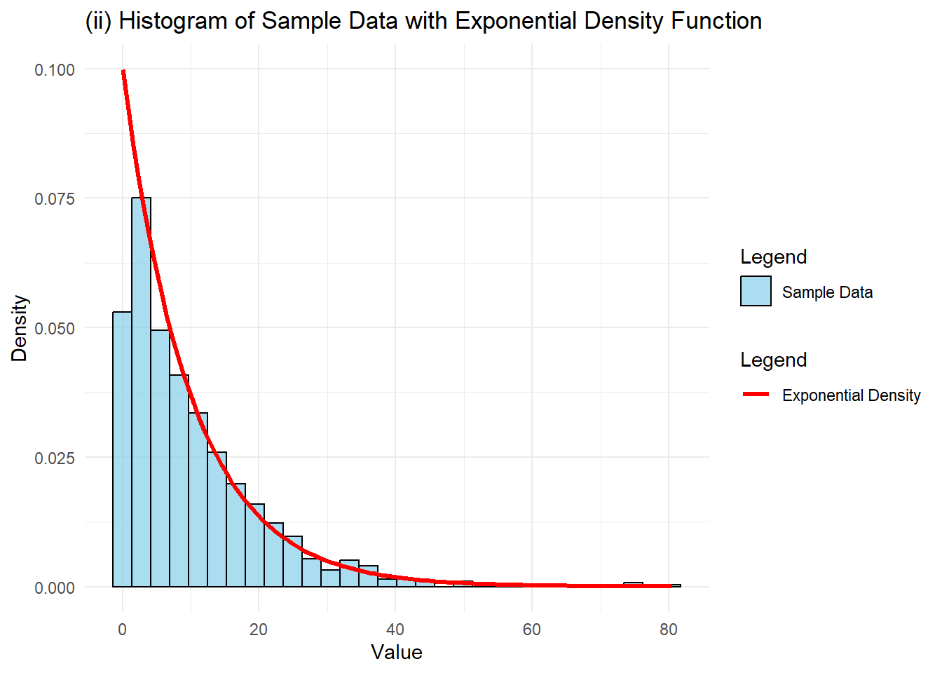
The generated data yielded a sample mean of 10.22 and sample standard deviation of 10.49. These values aligned closely with the population mean of 10 and population standard deviation of 10, as expected given the large sample size of 1000. The minor deviations stemmed from sampling randomness, but the sample estimates effectively approximated the theoretical population values.

The histogram of 1000 sample observations demonstrated strong alignment with the theoretical exponential distribution's shape, exhibiting pronounced right skewness. The overlaid red line, representing the theoretical density function with mean 10, closely matched the sample data histogram. This alignment illustrated how large samples accurately represented the underlying exponential distribution.

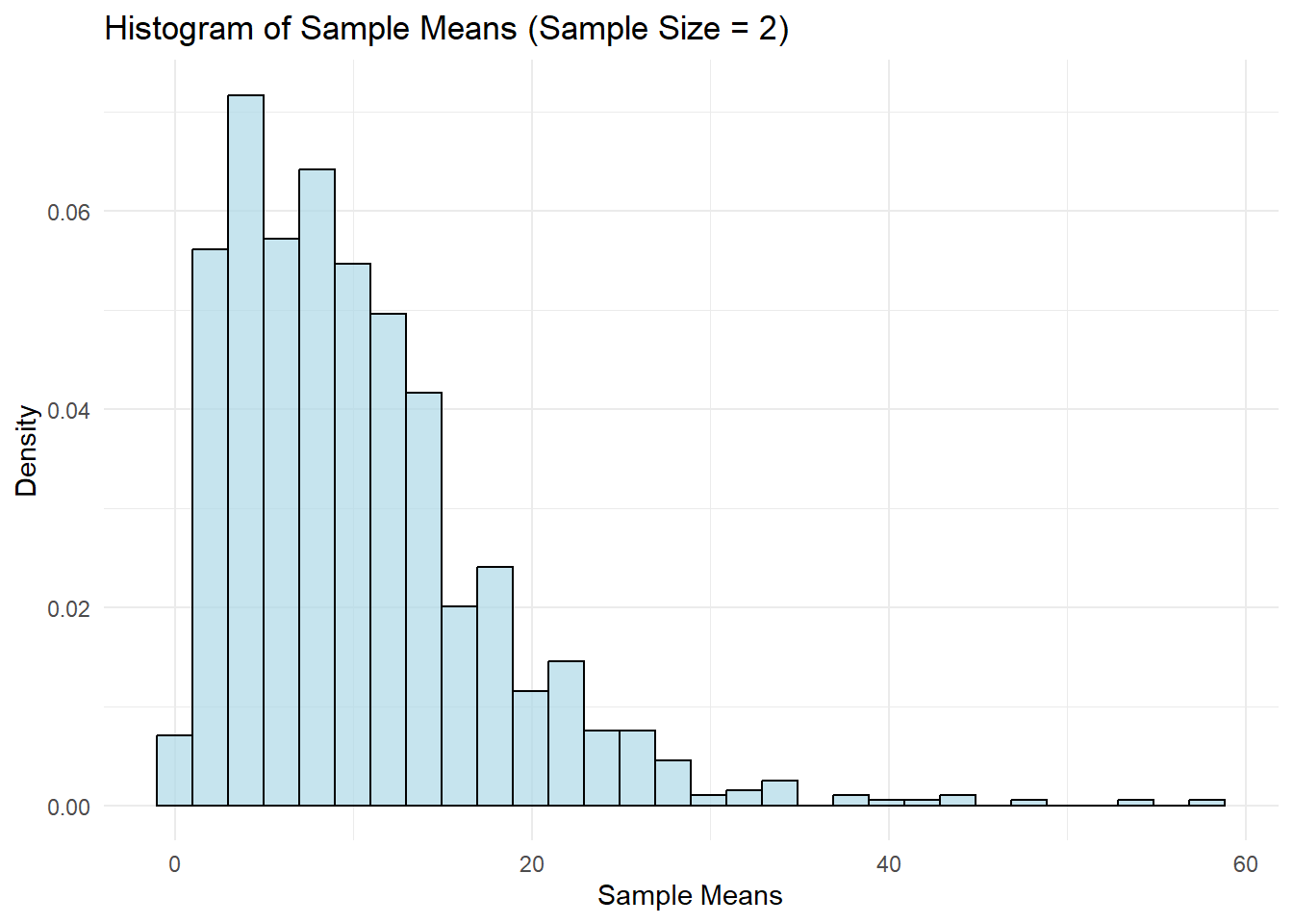
When examining sample means with a sample size of 2, the resulting histogram revealed a right-skewed distribution. The sample means showed substantial variability, with the distribution shape closely resembling the original exponential distribution. This behaviour emerged from the small sample size being insufficient to average out the inherent variability of the exponential distribution. The means exhibited considerable spread, reflecting the influence of the underlying skewed data.

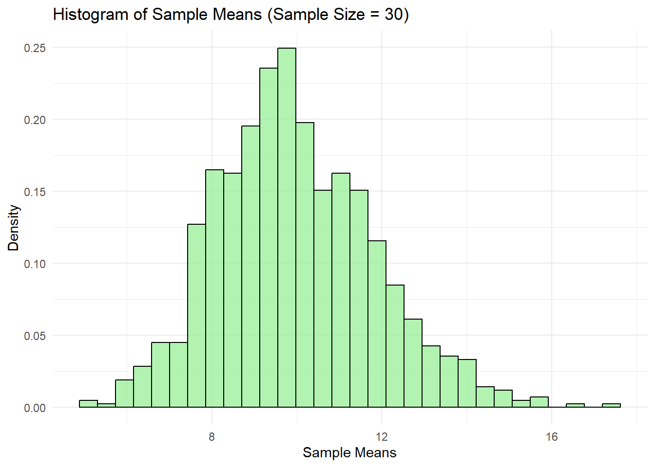
In contrast, the histogram of sample means with sample size 30 displayed a bell-shaped distribution approximating normality. This demonstrated the Central Limit Theorem (CLT), as the sample means' distribution approached normal form with increased sample size. The spread narrowed considerably compared to the sample size of 2, indicating how larger samples reduced variability and concentrated means around the population mean of 10.

Section 2: Summary and Clarification

The analysis demonstrated the Central Limit Theorem through the distribution of sample means. As sample sizes increased, the means became more stable and normally distributed. This principle proved valuable for understanding how sampling could be applied to estimate population parameters with enhanced accuracy in real-world scenarios.

Section 2: R Code Chunks

Sample Mean: 10.22

Sample Standard Deviation: 10.49

Population Mean: 10

Population Standard Deviation: 10

Section 3

Section 3: Analysis and Business Recommendations

a) One-Tailed t-Test Results:

The one-tailed t-test comparing the attractiveness of the current and new packaging designs yielded the following results:
- t-value: 1.65
- Critical t-value: 1.73
- p-value: 0.0579

The results indicated that the improvement in attractiveness score between the current design (mean = 7.5) and the new design (mean = 8.2) was not statistically significant at the 5% significance level.

Analysis Interpretation

Although participants rated the new design marginally higher, the statistical analysis demonstrated that this difference was not substantial enough to be considered significant. The observed improvement could have been attributed to chance rather than meaningful differences in the design changes.

The t-value (1.65) fell below the critical threshold (1.73), suggesting insufficient evidence to reject the null hypothesis of no difference between designs. The p-value of 0.0579 was slightly above the 0.05 threshold, indicating approximately 5.79% probability that the observed difference occurred by chance, placing it just outside statistical significance.

b) Recommendations and Next Steps:

The results warranted caution regarding major business decisions about the packaging redesign. While initial feedback suggested improved attractiveness, the statistical evidence was insufficient to justify the investment in a packaging overhaul.

Key considerations for management included:

• Statistical Significance : The improvement in attractiveness did not meet the 5% significance threshold. The difference could have been attributed to chance, making it difficult to confidently predict increased customer satisfaction or sales.

• Sample Size Considerations : A larger study with more participants could have reduced variability and potentially yielded significant results. However, there was no guarantee that increased sample size would have produced statistical significance. If the effect was genuinely small, a larger sample might have confirmed the improvement was not worth pursuing .

• Cost-Benefit Analysis : Given the data's uncertainty regarding substantial increases in sales or customer satisfaction, significant investment in redesign based solely on this limited study appeared unwise. The decision required careful consideration of financial and branding impacts against uncertain improvements in customer perception.

Section 3: Summary and Clarification

The new design demonstrated improvement, though statistical analysis revealed insufficient significance to warrant an overhaul. While a larger sample size might have provided more definitive results, this analysis suggested that investment in the new design might not have yielded substantial business benefits.

Final Note:

For continued interest in the new design, additional data collection or broader surveying would have been advisable to ensure the redesign would deliver positive and statistically significant impact before proceeding with large-scale changes.

Section 3: R Code Chunks

t-value: 1.65

Critical t-value: 1.73

p-value: 0.0579

Section 4

Section 4: Hypothesis Testing and Sample Comparison

The analysis examined two sample sizes to evaluate the impact of sample volume on hypothesis testing reliability.

For the initial test with 10 observations, the paired t-test yielded a p-value of 0.0279. This result led to the rejection of the null hypothesis at the 5% significance level, suggesting meaningful differences between the means despite the limited sample size. However, with fewer data points, the results remained more susceptible to individual variations.

The subsequent analysis of 30 observations produced a markedly lower p-value of 0.0019. This strengthened result reinforced the rejection of the null hypothesis and provided more robust evidence of the difference between means. The larger dataset offered greater statistical power and reduced the influence of outliers or random fluctuations.

Comparing the two analyses revealed the expected relationship between sample size and statistical confidence. The p-value decreased substantially from 0.0279 to 0.0019 as the sample size tripled, demonstrating enhanced detection capability. While both tests supported rejecting the null hypothesis, the larger sample delivered more definitive evidence of the underlying differences.

Section 4: Summary and Clarification

The investigation highlighted how increased sample sizes strengthened the ability to detect significant differences between paired groups. Though both analyses suggested meaningful variations existed, the larger sample provided more reliable insights into the true relationship between the populations studied. This reinforced the value of adequate sample sizes in hypothesis testing whilst acknowledging that smaller samples could still yield useful preliminary findings.

Section 4: R Code Chunks

Summary of Section 4 Results:

(a) Results for 10 observations:

p-value: 0.0279

Conclusion: Reject the null hypothesis

(b) Results for 30 observations:

p-value: 0.0019

(c) Comparison:

With a larger sample size, the test becomes more likely to detect a significant difference.

Section 5

Section 5: Analysis of Promotional Scenarios for Home Brand Chocolate Blocks

a) ANOVA Test with Standard Deviation of 30

The analysis employed a one-way ANOVA to examine sales performance across three promotional scenarios (Catalogue Only, End of Aisle, and Catalogue + Aisle). This statistical approach assessed potential differences between the group means.

F-statistic : 2.351 p-value : 0.129
With a p-value of 0.129 exceeding the 5% significance level, the analysis failed to reject the null hypothesis. The data revealed no significant variations in sales performance between the promotional strategies.

b) ANOVA Test with Standard Deviation of 25

A subsequent ANOVA utilising a reduced standard deviation of 25 yielded similar findings.

F-statistic : 2.31 p-value : 0.133
The data continued to support the initial conclusion: no single promotional strategy demonstrated superior sales performance.

c) Comparative Analysis

Both analyses arrived at consistent conclusions. The reduction in standard deviation produced minimal impact, with p-values remaining above 0.05. The statistical evidence suggested that the promotional strategies performed comparably in terms of sales generation.

Section 5: Summary and Clarification

The ANOVA analyses demonstrated comparable performance across all promotional strategies. The reduced standard deviation in the second test did not materially affect the outcomes. These findings suggested that alternative promotional approaches might warrant exploration to achieve meaningful sales improvements.

Section 5: R Code Chunks

Df Sum Sq Mean Sq F value Pr(>F)

Scenario 2 6811 3405 2.351 0.129

Residuals 15 21725 1448

Scenario 2 4647 2324 2.31 0.133

Residuals 15 15087 1006

References

Khan Academy 2024, Hypothesis testing and t-tests , viewed 21 September 2024, https://www.khanacademy.org/math/statistics-probability .

Statistics How To 2024, ANOVA Explained , viewed 21 September 2024, https://www.statisticshowto.com/probability-and-statistics .

Investopedia 2024, Central Limit Theorem , viewed 21 September 2024, https://www.investopedia.com/terms/c/central_limit_theorem.asp .

Wickham, H & Grolemund, G 2024, R for Data Science , viewed 21 September 2024, https://r4ds.had.co.nz .

R Code

library(dplyr)
library(ggplot2)
library(knitr)
library(tidyr)
library(MASS)

set.seed(3229642)

n_A <- 100  # Group A (Vaccinated)
n_B <- 100  # Group B (Placebo)

p_A <- 0.10  # Probability for Group A
p_B <- 0.30  # Probability for Group B

contract_flu_A <- rbinom(1, n_A, p_A)
contract_flu_B <- rbinom(1, n_B, p_B)

no_flu_A <- n_A - contract_flu_A
no_flu_B <- n_B - contract_flu_B

matrix_flu_table <- data.frame(
  Condition = c("Contracted the flu", "Did not contract the flu", "TOTAL"),
  Group_A = c(contract_flu_A, no_flu_A, n_A),
  Group_B = c(contract_flu_B, no_flu_B, n_B)
)

kable(matrix_flu_table, caption = "Flu Experiment Results: Matrix Format", col.names = c("Condition", "Group A", "Group B"))

prob_no_flu_B <- no_flu_B / n_B  # Keep this as a proportion for calculations
prob_no_flu_B_percent <- prob_no_flu_B * 100  # Convert to percentage for display

cat("(i) Estimated probability that a person in Group B (Placebo) did not contract the flu: ",
    round(prob_no_flu_B_percent, 2), "%", sep = "")

z_value <- 1.96  # Z value for 95% CI
std_error <- sqrt((prob_no_flu_B * (1 - prob_no_flu_B)) / n_B)

ci_lower <- prob_no_flu_B - z_value * std_error
ci_upper <- prob_no_flu_B + z_value * std_error

ci_lower_percent <- ci_lower * 100
ci_upper_percent <- ci_upper * 100

cat("(ii) 95% Confidence Interval for the proportion of people in Group B who did not contract the flu: ",
    round(ci_lower_percent, 2), "% to ", round(ci_upper_percent, 2), "%", sep = "")

p_A <- 0.10  # Probability of contracting the flu for vaccinated individuals
p_B <- 0.30  # Probability for non-vaccinated (placebo group)

p_flu_total <- 0.40 * p_A + 0.60 * p_B

p_flu_total_percent <- p_flu_total * 100

cat("(iii) Anticipated percentage of people in the wider population who will contract the flu: ",
    round(p_flu_total_percent, 2), "%", sep = "")

p_A <- 0.10

n_years <- 10

prob_3_or_more <- 1 - pbinom(2, size = n_years, prob = p_A)

cat("(iv) Estimated probability that a person vaccinated for ten years will contract the flu at least three times: ",
    round(prob_3_or_more * 100, 2), "%", sep = "")

set.seed(3229642)  # For reproducibility
lambda <- 0.1  # Rate parameter for exponential distribution (mean = 10)
n <- 1000  # Number of observations
sample_data <- rexp(n, rate = lambda)

sample_mean <- mean(sample_data)
sample_sd <- sd(sample_data)

pop_mean <- 10
pop_sd <- 10

cat("Sample Mean: ", round(sample_mean, 2), "\nSample Standard Deviation: ", round(sample_sd, 2), "\n")

cat("Population Mean: ", pop_mean, "\nPopulation Standard Deviation: ", pop_sd, "\n")

ggplot(data.frame(sample_data), aes(x = sample_data)) +
  geom_histogram(aes(y = ..density.., fill = "Sample Data"), bins = 30, color = "black", alpha = 0.7) +
  stat_function(fun = dexp, args = list(rate = lambda), aes(color = "Exponential Density"), size = 1.2) +
  scale_fill_manual(name = "Legend", values = c("Sample Data" = "skyblue")) +
  scale_color_manual(name = "Legend", values = c("Exponential Density" = "red")) +
  labs(title = "(ii) Histogram of Sample Data with Exponential Density Function",
       x = "Value", y = "Density") +
  theme_minimal()

set.seed(3229642)  # For reproducibility

n_samples <- 1000  # Number of sample means
sample_size <- 2  # Sample size for each mean

sample_means_2 <- replicate(n_samples, mean(rexp(sample_size, rate = lambda)))

ggplot(data.frame(sample_means_2), aes(x = sample_means_2)) +
  geom_histogram(aes(y = ..density..), bins = 30, fill = "lightblue", color = "black", alpha = 0.7) +
  labs(title = "Histogram of Sample Means (Sample Size = 2)",
       x = "Sample Means", y = "Density") +
  theme_minimal()

sample_size <- 30  # Sample size for each mean

sample_means_30 <- replicate(n_samples, mean(rexp(sample_size, rate = lambda)))

ggplot(data.frame(sample_means_30), aes(x = sample_means_30)) +
  geom_histogram(aes(y = ..density..), bins = 30, fill = "lightgreen", color = "black", alpha = 0.7) +
  labs(title = "Histogram of Sample Means (Sample Size = 30)",
       x = "Sample Means", y = "Density") +
  theme_minimal()

mean_old <- 7.5
mean_new <- 8.2
std_dev_diff <- 1.9
n <- 20  # Sample size

t_value <- (mean_new - mean_old) / (std_dev_diff / sqrt(n))

df <- n - 1

alpha <- 0.05
t_critical <- qt(1 - alpha, df)

p_value <- pt(t_value, df, lower.tail = FALSE)

cat("t-value: ", round(t_value, 2), "\n")

cat("Critical t-value: ", round(t_critical, 2), "\n")

cat("p-value: ", round(p_value, 4), "\n")

set.seed(3229642)

mu1 <- 50   # Mean of the first variable
mu2 <- 55   # Mean of the second variable
sigma1 <- 10  # Standard deviation of the first variable
sigma2 <- 10  # Standard deviation of the second variable
rho <- 0.8  # Correlation coefficient

cov_matrix <- matrix(c(sigma1^2, rho * sigma1 * sigma2, rho * sigma1 * sigma2, sigma2^2), nrow=2)

data_10 <- mvrnorm(n=10, mu=c(mu1, mu2), Sigma=cov_matrix)

x_10 <- data_10[, 1]  # First variable
y_10 <- data_10[, 2]  # Second variable
t_test_10 <- t.test(x_10, y_10, paired=TRUE)

p_value_10 <- round(t_test_10$p.value, 4)
result_10 <- ifelse(p_value_10 < 0.05, "Reject the null hypothesis", "Fail to reject the null hypothesis")

data_30 <- mvrnorm(n=30, mu=c(mu1, mu2), Sigma=cov_matrix)

x_30 <- data_30[, 1]  # First variable
y_30 <- data_30[, 2]  # Second variable
t_test_30 <- t.test(x_30, y_30, paired=TRUE)

p_value_30 <- round(t_test_30$p.value, 4)
result_30 <- ifelse(p_value_30 < 0.05, "Reject the null hypothesis", "Fail to reject the null hypothesis")

comparison <- ifelse(p_value_30 < p_value_10,
                     "With a larger sample size, the test becomes more likely to detect a significant difference.",
                     "Increasing the sample size does not always lead to a more significant result.")

cat("
Summary of Section 4 Results:

(a) Results for 10 observations:
p-value: ", p_value_10, "\nConclusion: ", result_10, "

(b) Results for 30 observations:
p-value: ", p_value_30, "\nConclusion: ", result_30, "

(c) Comparison:
", comparison, "\n")

set.seed(3229642)

n_stores <- 6

mean_scenario1 <- 50
mean_scenario2 <- 55
mean_scenario3 <- 60
sd_scenario <- 30  # standard deviation

sales_scenario1 <- rnorm(n_stores, mean = mean_scenario1, sd = sd_scenario)
sales_scenario2 <- rnorm(n_stores, mean = mean_scenario2, sd = sd_scenario)
sales_scenario3 <- rnorm(n_stores, mean = mean_scenario3, sd = sd_scenario)

sales_data <- data.frame(
  Scenario = rep(c("Catalogue Only", "End of Aisle", "Catalogue + Aisle"), each = n_stores),
  Sales = c(sales_scenario1, sales_scenario2, sales_scenario3)
)

anova_result <- aov(Sales ~ Scenario, data = sales_data)

summary(anova_result)

sd_sales_new <- 25

set.seed(3229642)
sales_data_new <- data.frame(
  Scenario = rep(c("Catalogue Only", "End of Aisle", "Catalogue + Aisle"), each = 6),
  Sales = c(
    rnorm(6, mean = 50, sd = sd_sales_new),
    rnorm(6, mean = 55, sd = sd_sales_new),
    rnorm(6, mean = 60, sd = sd_sales_new)
  )
)

anova_result_new <- aov(Sales ~ Scenario, data = sales_data_new)

summary(anova_result_new)