Streaming Recommendation Engine
Fair warning: These posts are super dry because they are academic papers. Sorry!
Investigating the Impact of a New Recommendation Engine on Streaming Engagement
A Data-Driven Analysis for ‘Why Not Watch?’
Kip Jordan
A statistical analysis conducted as part of the Data Science Graduate Certificate at RMIT University, Melbourne, Australia
Introduction
In today's data-driven world, optimising user engagement is key to maintaining a competitive edge. To address this, 'Why Not Watch?' introduced a new recommendation engine to see if it could improve user engagement. This presentation will focus on evaluating whether the new engine has increased the number of hours users spend watching content. Our analysis revolves around comparing two user groups: those exposed to the new engine (Group B) and those using the previous version (Group A).
This analysis will help the executive team determine whether rolling out the new recommendation engine to the entire user base is justified, based on clear, actionable insights from the data.
Objective: Measure the impact of the new recommendation engine on user engagement.
Metric of Interest: Hours watched per user.
Approach: Statistical analysis of A/B testing data to compare the two user groups.
Goal: Provide clear recommendations for the potential rollout of the new engine.
Problem Statement
The core problem driving our investigation is whether the new recommendation engine has succeeded in increasing user engagement. Specifically, the question we're asking is: Does Group B, who used the new recommendation engine, engage with more content (measured in hours watched) than Group A, who used the old engine?
To answer this, we employed statistical tools to compare these two groups and determine the effectiveness of the new engine. By carefully accounting for factors such as age and social engagement, we've minimised bias to ensure our results are valid and actionable for decision-making.
Problem: Is the new recommendation engine increasing user engagement?
Approach: Statistical comparison of hours watched between Group A (control) and Group B (new engine).
Focus: Minimise bias by controlling for key variables like age and social engagement, ensuring that the results are robust and reliable.
Data
To properly assess the impact of the new recommendation engine, we worked with a comprehensive dataset provided by 'Why Not Watch?', which contained all the necessary information from the A/B test. The dataset includes detailed information about each user's behaviour, demographics, and interaction with the recommendation engine.
The key variables used in our analysis include:
Group:
- Categorical variable representing the user group
- Levels:
- A: Users in the control group (old recommendation engine)
- B: Users in the treatment group (new recommendation engine)
Age:
- Numeric variable representing the user's age
- Scale: The values range from 18 to 55, with a mean of 36.49
Social Metric:
- Numeric variable summarising the user's engagement with social features on the platform
- Scale: A score between 0 and 10, with a mean of 4.91
Hours Watched:
- The main dependent variable, representing the number of hours the user spent watching content during the test period
- Scale: Measured in hours, with values ranging from 0.5 to 8.3 hours, and a mean of 4.39 hours
Demographic:
- Categorical variable representing the user's demographic group
- Levels: 1 to 4 (representing different demographic categories)
Gender:
- Categorical variable
- Levels:
- F: Female
- M: Male
Time Since Signup:
- Numeric variable representing how long the user has been subscribed to the platform
- Scale: Measured in months, with values ranging from 0 to 24 months, with a mean of 11.97 months
Data Summary
As a follow-up to the previous breakdown of key variables, this slide provides a more detailed summary of the dataset. Here, we display the full structure and statistical summaries of the data, showcasing all eight variables used in the analysis. This summary allows us to better understand the distributions, ranges, and key metrics, such as the mean and median, for each variable. It also helps to identify patterns and distributions that will be explored further in the analysis.
The table on the top outlines the structure of the dataset, including the data types and first few observations of each variable. The table below offers a detailed summary of the numeric variables, including measures like the minimum, maximum, and mean for age, hours_watched, social_metric, and others.
| Statistic | Value |
|---|---|
| 'data.frame' | 1000 obs. of 8 variables: |
| $ date | chr "1-Jul" "1-Jul" "1-Jul" "1-Jul" ... |
| $ gender | chr "F" "F" "F" "M" ... |
| $ age | int 28 32 39 52 25 51 53 42 41 20 ... |
| $ social_metric | int 5 7 4 10 1 0 5 6 8 7 ... |
| $ time_since_signup | num 19.3 11.5 4.3 9.5 19.5 22.6 4.2 8.5 16.9 23 ... |
| $ demographic | int 1 1 3 4 2 4 3 4 4 2 ... |
| $ group | chr "A" "A" "A" "A" ... |
| $ hours_watched | num 4.08 2.99 5.74 4.13 4.68 3.4 3.07 2.77 2.24 5.39 ... |
| Statistic | Value |
|---|---|
| date gender age social_metric | - |
| Length | 1000 Length:1000 Min. :18.00 Min. : 0.000 |
| Class | character Class :character 1st Qu.:28.00 1st Qu.: 2.000 |
| Mode | character Mode :character Median :36.00 Median : 5.000 |
| Mean | 36.49 Mean : 4.911 |
| 3rd Qu. | 46.00 3rd Qu.: 8.000 |
| Max. | 55.00 Max. :10.000 |
| time_since_signup demographic group hours_watched | - |
| Min. | 0.00 Min. :1.000 Length:1000 Min. :0.500 |
| 1st Qu. | 5.70 1st Qu.:2.000 Class :character 1st Qu.:3.530 |
| Median | 11.80 Median :3.000 Mode :character Median :4.415 |
| Mean | 11.97 Mean :2.603 Mean :4.393 |
| 3rd Qu. | 18.70 3rd Qu.:4.000 3rd Qu.:5.322 |
| Max. | 24.00 Max. :4.000 Max. :8.300 |
Data Preprocessing
To ensure that the analysis was reliable and free from errors, we began by carefully cleaning and preparing the dataset. This involved removing any missing values (NAs), as they could skew the results. For instance, we specifically filtered out users with missing hours_watched data, as this was our primary measure of engagement.
Additionally, we converted key categorical variables—such as group, gender, and demographic—into factors, allowing us to properly analyse them during our statistical tests. One critical issue we identified early on was a potential bias due to unequal age distributions between the groups: Group A had an older average age than Group B. To minimise the risk of this age imbalance distorting our findings, we controlled for age during our regression and ANOVA analysis.
Key Points:
- Cleaning Steps:
- Removed rows with missing values (NA) in hours_watched
- Converted categorical variables (group, gender, demographic) to factors
- Bias Identification: Group A was older on average, which could introduce bias
- Correction: We controlled for age in the statistical models to ensure unbiased results
These preprocessing steps, particularly the handling of missing values and categorical variables, were essential to ensure that our regression and t-test analyses are both valid and unbiased. Additionally, by controlling for age imbalances between groups, we can confidently interpret the model results in the next sections.
Data Preprocessing and Normality Check
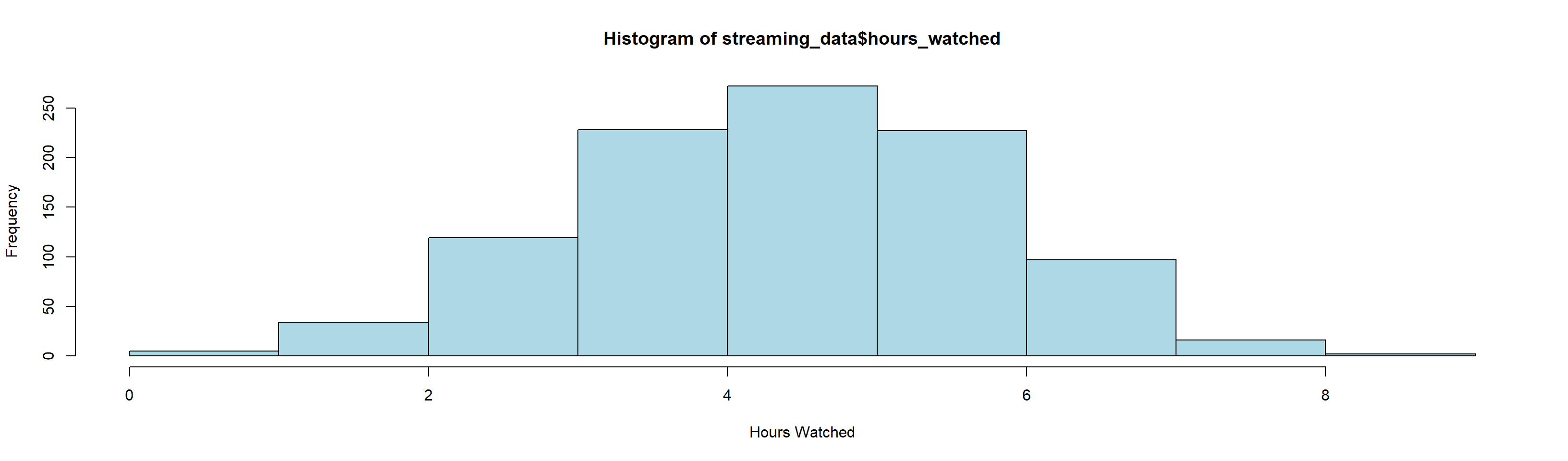
After cleaning the data, we needed to ensure that the key variables conformed to the assumptions necessary for valid statistical testing. In particular, checking for normality in hours watched ensures that the parametric tests we perform later, like the t-test and regression, are appropriate and reliable.
Histogram of Hours Watched
Shapiro-Wilk normality test
| Statistic | Value |
|---|---|
| Test Type | Shapiro-Wilk normality test |
| Data | streaming_data$hours_watched |
| W-statistic | 0.99792 |
| p-value | 0.2495 |
The Shapiro-Wilk test confirmed that the distribution of hours watched did not significantly deviate from normality (p > 0.05), allowing us to proceed with parametric statistical analyses.
Analysis: T-Test Results for Hours Watched Between Groups A and B
We begin our analysis with a high-level comparison of hours watched between Group A and Group B using a Welch two-sample t-test. This provides an initial indication of whether the new recommendation engine has significantly impacted user engagement.
The Welch two-sample t-test was used to assess whether the new recommendation engine (Group B) increased engagement compared to the old engine (Group A). The test showed a significant difference between the two groups (p < 0.001), suggesting that users exposed to the new recommendation engine watched more hours of content on average.
| Statistic | Value |
|---|---|
| Test Type | Welch Two Sample t-test |
| Data | hours_watched by group |
| Test Statistics | t = -3.672, df = 153.01, p-value = 0.000332 |
| Alternative Hypothesis | true difference in means between group A and group B is not equal to 0 |
| 95% Confidence Interval | -0.7301713 to -0.2193287 |
| Sample Estimates | mean in group A: 4.336125 |
| mean in group B: 4.810875 |
Analysis: Initial Regression Analysis
While the t-test provides an initial indication of the new recommendation engine's effectiveness, it's essential to account for other factors, such as age and social engagement. To quantify the influence of these variables, we conducted a regression analysis, examining key factors like age, social_metric, group, time since signup, gender, and demographic to determine which significantly impact hours watched.
Key Variables:
Dependent Variable: Hours Watched
Independent Variables: Age, Social Metric, Group, Gender, Demographic, Time Since Signup
| Variable | Estimate | Std. Error | t value | p-value |
|---|---|---|---|---|
| (Intercept) | 6.299174 | 0.196633 | 32.035 | < 2e-16 *** |
| age | -0.065189 | 0.006017 | -10.834 | < 2e-16 *** |
| social_metric | 0.095349 | 0.010961 | 8.699 | < 2e-16 *** |
| time_since_signup | 0.003503 | 0.004543 | 0.771 | 0.441 |
| groupB | 0.642787 | 0.102245 | 6.287 | 4.85e-10 *** |
| genderM | -0.182936 | 0.142600 | -1.283 | 0.200 |
| demographic2 | 0.145210 | 0.139705 | 1.039 | 0.299 |
| demographic3 | -0.231789 | 0.150630 | -1.539 | 0.124 |
Model Statistics:
- Residual standard error: 1.034 on 992 degrees of freedom
- Multiple R-squared: 0.4023, Adjusted R-squared: 0.3981
- F-statistic: 95.37 on 7 and 992 DF, p-value: < 2.2e-16
Significance codes: 0 '' 0.001 '' 0.01 '' 0.05 '.' 0.1 ' ' 1
Analysis: Initial Regression Analysis Visualisation
This visualisation complements the findings from our initial regression analysis. It illustrates the relationships between hours watched and key independent variables such as age, social metric, and group.
Age vs Hours Watched: We observe a negative trend, particularly for Group A (control group), where older users tend to watch fewer hours. The trend is less steep for Group B (treated group), suggesting that the new recommendation engine may mitigate the effect of age on engagement.
Social Metric vs Hours Watched: As expected, higher social engagement (measured through the social metric) correlates positively with hours watched. Group B shows a steeper increase in hours watched as social engagement rises, indicating a more effective impact from the recommendation engine in this group.
Group vs Hours Watched: The box plot further highlights that Group B consistently watches more hours than Group A, supporting the hypothesis that the new recommendation engine has increased engagement overall.
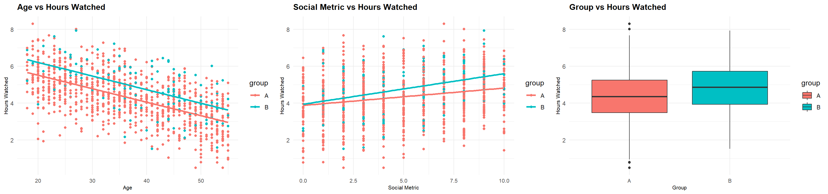
These visualisations reinforce the key takeaways from our regression model, indicating significant effects from age, social engagement, and group assignment on the dependent variable, hours watched.
This visual evidence aligns with our hypothesis: the new recommendation engine appears to mitigate age-related declines in engagement and more effectively boosts hours watched as social engagement increases.
Analysis: ANOVA Results Considering Age, Group, and Social Engagement
While the t-test identified significant differences in hours watched, the ANOVA allowed us to explore how various factors—like age, social engagement, and group—contribute to engagement. This model confirmed that both age and group were significant predictors.
| Term | Df | Sum Sq | Mean Sq | F value | Pr(>F) |
|---|---|---|---|---|---|
| age | 1 | 582.6 | 582.6 | 544.605 | < 2e-16 *** |
| social_metric | 1 | 85.2 | 85.2 | 79.684 | < 2e-16 *** |
| time_since_signup | 1 | 0.3 | 0.3 | 0.244 | 0.622 |
| group | 1 | 43.5 | 43.5 | 40.690 | 2.73e-10 *** |
| gender | 1 | 0.0 | 0.0 | 0.000 | 0.983 |
| demographic | 2 | 2.6 | 1.3 | 1.198 | 0.302 |
| Residuals | 992 | 1061.2 | 1.1 | ||
| ------------------- | ----- | --------- | --------- | --------- | ----------- |
| Signif. codes: | 0 '' 0.001 '' 0.01 '' 0.05 '.' 0.1 ' ' 1 |
The ANOVA results reinforce the findings from our regression analysis, with a significant interaction between social engagement and group assignment, confirming that the recommendation engine's impact was stronger for more socially engaged users.
Analysis: Age Bias in Groups
While analysing the data, we discovered a potential bias in age distribution between the two groups. Group B, exposed to the new recommendation engine, was significantly younger, which might have influenced their engagement independently of the recommendation engine. To test this, we performed a t-test to compare the average ages of the two groups.
Assumptions Checked:
- Normality of data
- Equal variances between groups
| Statistic | Value |
|---|---|
| Welch Two Sample t-test (Age) | |
| Data | age by group |
| t-statistic | -2.8185 |
| Degrees of freedom | 157.95 |
| p-value | 0.005443 |
| Alternative hypothesis | true difference in means between group A and group B is not equal to 0 |
| 95% confidence interval | [-4.7460366, -0.8350241] |
| Sample estimates | |
| Mean in group A | 36.15114 |
| Mean in group B | 38.94167 |
| Statistic | Value |
|---|---|
| Welch Two Sample t-test (Social Metric) | |
| Data | social_metric by group |
| t-statistic | -1.2752 |
| Degrees of freedom | 157.33 |
| p-value | 0.2041 |
| Alternative hypothesis | true difference in means between group A and group B is not equal to 0 |
| 95% confidence interval | [-0.9095148, 0.1958784] |
| Sample estimates | |
| Mean in group A | 4.868182 |
| Mean in group B | 5.225000 |
Interpretation: The t-test confirmed a significant difference in age between the two groups (p-value < 0.05), indicating the need to control for age in further analysis.
Analysis: Adjusting for Age and Social Engagement in the Regression Model
Given the significant age imbalance between Groups A and B, it was essential to adjust our regression model to accurately capture the effects of age and social engagement on hours watched. To ensure that differences in engagement between the two groups were not merely driven by age, we introduced interaction terms between age and group.
| Statistic | Value |
|---|---|
| Call | lm(formula = hours_watched ~ age + social_metric + group + age:group + |
| social_metric:group, data = streaming_data) | |
| --------------------------- | --------------------------------------------------------------------------------- |
| Residuals | |
| Min 1Q Median | -3.6244 -0.6323 -0.0218 0.6988 2.8773 |
| --------------------------- | --------------------------------------------------------------------------------- |
| Coefficients | Estimate Std. Error t value Pr(> |
| (Intercept) | 6.535941 0.136392 47.920 < 2e-16 *** |
| age | -0.072279 0.003244 -22.279 < 2e-16 *** |
| social_metric | 0.084869 0.011555 7.345 4.28e-13 *** |
| groupB | 0.304804 0.430690 0.708 0.47929 |
| age:groupB | -0.003504 0.009916 -0.353 0.72391 |
| social_metric:groupB | 0.091444 0.035078 2.607 0.00927 ** |
| --------------------------- | --------------------------------------------------------------------------------- |
| Signif. codes: | 0 '' 0.001 '' 0.01 '' 0.05 '.' 0.1 ' ' 1 |
| --------------------------- | --------------------------------------------------------------------------------- |
| Residual standard error | 1.031 on 994 degrees of freedom |
| Multiple R-squared | 0.4047, Adjusted R-squared: 0.4017 |
| F-statistic | 135.1 on 5 and 994 DF, p-value: < 2.2e-16 |
The results of this adjusted model indicate that while age remains a significant predictor of hours watched, the new recommendation engine did not interact significantly with age. However, social engagement (social_metric) showed a stronger interaction with the recommendation engine, suggesting that users with higher social engagement in Group B watched more content.
Analysis: Adjusting for Age and Social Engagement in the ANOVA Model
After adjusting for age in our regression model, we conducted an ANOVA with interaction terms to further validate our findings. The ANOVA breaks down the variance in hours watched and shows how multiple factors, including age, social engagement, and group, contribute to the observed differences in engagement.
| Statistic | Df | Sum Sq | Mean Sq | F value | Pr(>F) |
|---|---|---|---|---|---|
| age | 1 | 582.6 | 582.6 | 547.895 | < 2e-16 *** |
| group | 1 | 48.3 | 48.3 | 45.460 | 2.64e-11 *** |
| social_metric | 1 | 80.2 | 80.2 | 75.422 | < 2e-16 *** |
| age:group | 1 | 0.1 | 0.1 | 0.073 | 0.78695 |
| group:social_metric | 1 | 7.2 | 7.2 | 6.796 | 0.00927 ** |
| Residuals | 994 | 1057.0 | 1.1 | ||
| --------------------------- | --------- | --------- | --------- | --------- | ------------ |
| Signif. codes: | 0 '***' | 0.001 '**' | 0.01 '*' | 0.05 '.' | 0.1 ' ' 1 |
Importantly, the interaction between group and social engagement was again significant (p < 0.01), indicating that users with higher social engagement in Group B watched significantly more hours of content. However, the interaction between age and group was not significant (p = 0.78695), further confirming that age did not strongly influence the effect of the new recommendation engine.
Discussion
Major Findings
The analysis shows that the new recommendation engine had a statistically significant impact on user engagement, with Group B (who used the new engine) watching more hours of content than Group A (who used the old engine). While the t-test initially highlighted this difference, regression analysis confirmed that age and social engagement were also significant factors influencing hours watched. Most notably, the interaction between social engagement and group assignment indicated that the effectiveness of the recommendation engine was greater for users with higher levels of social engagement. This suggests that socially engaged users benefited more from the new recommendation system, leading to increased streaming activity.
Strengths and Limitations
A key strength of this investigation was the rigorous control for potential biases, particularly the identified age imbalance between the two groups. By introducing interaction terms in the regression model, we were able to minimise the risk of age differences affecting the results, ensuring that the observed effects were largely driven by the recommendation engine and not by demographic factors. However, a limitation of this analysis is that it focused exclusively on hours watched as a measure of engagement. Other potential metrics, such as content variety or frequency of return visits, were not considered but could provide a broader understanding of user behaviour in future studies.
Future Directions
To build on these findings, future investigations should consider incorporating additional metrics to capture a more comprehensive view of user engagement. For instance, analysing the variety of content consumed or the frequency of return visits could offer further insights into how the recommendation engine affects long-term user retention. Additionally, exploring how other user demographics (e.g., geographic location, income level) interact with the recommendation engine could provide valuable data for optimising the system for different segments of the user base.
Conclusion
In conclusion, this analysis provides clear evidence that the new recommendation engine has successfully increased user engagement, particularly among socially active users. By accounting for biases such as age and controlling for key variables, we have demonstrated that the engine's impact is both significant and meaningful. The findings support the recommendation to roll out the new engine to a broader audience, with the potential to drive higher engagement and content consumption across the platform.
References
R Libraries and Documentation:
Wickham, H. & Chang, W., 2023. ggplot2: Elegant Graphics for Data Analysis. Available at: https://ggplot2.tidyverse.org [Accessed 6 October 2024].
Wickham, H., François, R., Henry, L. & Müller, K., 2023. dplyr: A Grammar of Data Manipulation. Available at: https://dplyr.tidyverse.org [Accessed 6 October 2024].
Xie, Y., 2023. knitr: A General-Purpose Package for Dynamic Report Generation in R. Available at: https://yihui.org/knitr/ [Accessed 6 October 2024].
Auguie, B., 2017. gridExtra: Miscellaneous Functions for "Grid" Graphics. Available at: https://cran.r-project.org/web/packages/gridExtra/index.html [Accessed 6 October 2024].
Statistical Methods:
Welch, B.L., 1947. The generalization of 'Student's' problem when several different population variances are involved. Biometrika, 34(1-2), pp.28-35. Available at: https://www.statisticshowto.com/welchs-t-test-definition-examples/ [Accessed 6 October 2024].
University of California, Irvine, n.d. Linear Regression in R. Available at: https://stats.idre.ucla.edu/r/dae/linear-regression-in-r/ [Accessed 6 October 2024].
CRAN, n.d. ANOVA (Analysis of Variance) in R. Available at: https://cran.r-project.org/web/packages/easyanova/index.html [Accessed 6 October 2024].
RMarkdown and Slidy Presentation:
Xie, Y., 2023. RMarkdown: Dynamic Documents for R. Available at: https://rmarkdown.rstudio.com [Accessed 6 October 2024].
Xie, Y., 2023. Slidy Presentations with RMarkdown. Available at: https://bookdown.org/yihui/rmarkdown/slidy-presentation.html [Accessed 6 October 2024].
Dataset:
RMIT University, 2024. Streaming Engagement Dataset. Provided for educational purposes as part of Data Analytics assignment. [Accessed 6 October 2024].