Synthetic Data Generation
Fair warning: These posts are super dry because they are academic papers. Sorry!
A Synthetic Analysis of Ride-Sharing Service Data
Kip Jordan
A statistical analysis conducted as part of the Data Science Graduate Certificate at RMIT University, Melbourne, Australia
Project Overview
This project demonstrates techniques for generating and working with synthetic data in R, using a ride-sharing service scenario as an example. The aim was to create realistic, interconnected datasets that could be used to practise data wrangling and analysis techniques.
Key aspects of this project include:
- Generation of synthetic data with realistic properties and relationships
- Creation of multiple related datasets that can be merged and analysed
- Introduction of common data quality issues like missing values and outliers
- Implementation of data preprocessing and cleaning techniques
The project serves as a practical example of how to create test data that maintains logical consistency whilst incorporating real-world data characteristics. This synthetic data generation approach is valuable for:
- Testing data processing pipelines
- Developing and validating analysis methods
- Teaching and learning data science concepts
- Prototyping solutions without using sensitive production data
Data Description
I created synthetic data to simulate Uber's ride-sharing service operations. Here we generated two primary datasets to represent typical ride-sharing data structures:
Driver Dataset (50 records):
- driver_id: Unique identifier for each driver
- driver_name: Randomly generated driver names
- vehicle_type: Vehicle categories (Sedan, SUV, Premium)
- driver_rating: Rating scores between 3.5 and 5.0
- join_date: Dates throughout 2023 when drivers joined the platform
Ride Details Dataset (75 records):
- ride_id: Unique identifier for each ride
- driver_id: Links to the driver dataset
- trip_distance: Distance in kilometers (correlated with fare)
- fare_amount: Trip cost (based on distance plus base rate)
- payment_method: Payment type (Card, Cash, Digital Wallet)
- ride_date: Dates in early 2024 when rides occurred
The data includes realistic features such as:
- Correlated variables (trip distance and fare amount)
- Missing values (3 in each dataset)
- Outliers in numeric variables (ratings, fares, and distances)
- A mix of data types (numeric, categorical, dates)
Sample rows from Driver Dataset:
| driver_id | driver_name | vehicle_type | driver_rating | join_date | |
|---|---|---|---|---|---|
| 1 | S9700 | SUV | 3.76 | 2023-06-24 | |
| 2 | J3582 | Premium | 4.27 | 2023-11-17 | |
| 3 | Y9938 | Premium | 3.95 | 2023-08-26 | |
| 4 | Q8007 | SUV | 4.20 | 2023-05-17 | |
| 5 | R1410 | SUV | 3.58 | 2023-01-19 | |
| 6 | R9173 | SUV | 3.97 | 2023-12-31 |
Sample rows from Ride Details Dataset:
| ride_id | driver_id | trip_distance | fare_amount | payment_method | ride_date | |
|---|---|---|---|---|---|---|
| 1 | 46 | 6.35 | 16.94 | Cash | 2024-01-18 | |
| 2 | 36 | 18.42 | 36.87 | Card | 2024-02-08 | |
| 3 | 45 | 18.97 | 43.86 | Card | 2024-02-24 | |
| 4 | 49 | 15.69 | 39.18 | Cash | 2024-01-16 | |
| 5 | 15 | 9.06 | 20.09 | Cash | 2024-01-30 | |
| 6 | 47 | 4.70 | 12.66 | Card | 2024-01-11 |
Merge
I merged the two datasets using the common driver_id field as the key. Here we performed a left join to ensure all rides were retained while matching them with their corresponding driver information. I chose this approach as it's logical for a ride-sharing service where every ride must have an associated driver.
The columns were then reordered to improve readability, placing:
- Identifying information first (ride_id, driver_id, driver_name)
- Driver characteristics (vehicle_type, rating)
- Ride-specific details (distance, fare, payment_method, and dates)
The merged dataset contains 75 rows (matching our ride records) and 10 columns, combining all relevant information from both source datasets. This merged dataset was exported to Excel for documentation purposes.
Input dataset dimensions:
- Rides dataset: 75 rows by 6 columns
- Drivers dataset: 50 rows by 5 columns
Output dataset dimensions:
- Merged dataset: 75 rows by 10 columns
| ride_id | driver_id | driver_name | vehicle_type | driver_rating | trip_distance | fare_amount | payment_method | ride_date | join_date | |
|---|---|---|---|---|---|---|---|---|---|---|
| 1 | 46 | M9325 | Premium | 4.92 | 6.35 | 16.94 | Cash | 2024-01-18 | 2023-08-17 | |
| 2 | 36 | O3996 | SUV | NA | 18.42 | 36.87 | Card | 2024-02-08 | 2023-06-06 | |
| 3 | 45 | E3108 | Sedan | 3.56 | 18.97 | 43.86 | Card | 2024-02-24 | 2023-05-18 | |
| 4 | 49 | I8972 | Sedan | 4.34 | 15.69 | 39.18 | Cash | 2024-01-16 | 2023-09-23 | |
| 5 | 15 | P1728 | Sedan | 3.79 | 9.06 | 20.09 | Cash | 2024-01-30 | 2023-05-07 | |
| 6 | 47 | K2411 | SUV | 4.38 | 4.70 | 12.66 | Card | 2024-01-11 | 2023-10-28 |
Understand
I examined the merged dataset to understand its structure and ensure appropriate data types were assigned. My initial inspection revealed a mix of character and numeric variables that required optimisation. Here we converted categorical variables (vehicle_type and payment_method) to factors to improve memory efficiency and ensure proper categorical handling in analyses.
Date fields were verified to confirm proper formatting and logical ranges, with ride dates falling in early 2024 and join dates throughout 2023. The data structure inspection confirmed 10 variables with appropriate types for their content.
| Variable | Details | Summary Statistics |
|---|---|---|
| ride_id | Integer | Min: 1.0 1st Qu: 19.5 Median: 38.0 Mean: 38.0 3rd Qu: 56.5 Max: 75.0 |
| driver_id | Integer | Min: 2.00 1st Qu: 15.00 Median: 23.00 Mean: 25.36 3rd Qu: 37.50 Max: 50.00 |
| driver_name | Character | Length: 75 Class: character Mode: character |
| vehicle_type | Factor (3 levels) | Levels: "Premium", "Sedan", "SUV" |
| driver_rating | Numeric | Min: 3.560 1st Qu: 3.825 Median: 4.310 Mean: 4.281 3rd Qu: 4.718 Max: 4.980 NA's: 9 |
| trip_distance | Numeric | Min: 2.500 1st Qu: 6.965 Median: 11.470 Mean: 11.901 3rd Qu: 16.025 Max: 50.000 |
| fare_amount | Numeric | Min: 8.90 1st Qu: 17.20 Median: 28.43 Mean: 29.24 3rd Qu: 37.57 Max: 150.00 NA's: 3 |
| payment_method | Factor (3 levels) | Levels: "Card", "Cash", "Digital Wallet" |
| ride_date | Date | Min: 2024-01-01 1st Qu: 2024-01-15 Median: 2024-01-29 Mean: 2024-01-28 3rd Qu: 2024-02-09 Max: 2024-03-01 |
| join_date | Date | Min: 2023-01-24 1st Qu: 2023-05-08 Median: 2023-06-26 Mean: 2023-07-13 3rd Qu: 2023-08-19 Max: 2023-12-31 |
Manipulate Data
To enhance our analysis capabilities, I created several derived variables from the existing data. Here we calculated a driver experience metric as the number of days between each ride_date and the driver's join_date, providing insight into driver tenure.
I analysed fare efficiency through a fare-per-kilometre calculation, while estimated trip durations were computed assuming an average urban speed of 30 km/h.
Here's a sample of the enhanced dataset with the derived variables:
| ride_id | driver_id | driver_name | vehicle_type | driver_rating | trip_distance | fare_amount | payment_method | ride_date | join_date | driver_experience_days | fare_per_km | estimated_duration_mins | |
|---|---|---|---|---|---|---|---|---|---|---|---|---|---|
| 1 | 46 | M9325 | Premium | 4.92 | 6.35 | 16.94 | Cash | 2024-01-18 | 2023-08-17 | 154 | 2.67 | 13 | |
| 2 | 36 | O3996 | SUV | NA | 18.42 | 36.87 | Card | 2024-02-08 | 2023-06-06 | 247 | 2.00 | 37 | |
| 3 | 45 | E3108 | Sedan | 3.56 | 18.97 | 43.86 | Card | 2024-02-24 | 2023-05-18 | 282 | 2.31 | 38 | |
| 4 | 49 | I8972 | Sedan | 4.34 | 15.69 | 39.18 | Cash | 2024-01-16 | 2023-09-23 | 115 | 2.50 | 31 | |
| 5 | 15 | P1728 | Sedan | 3.79 | 9.06 | 20.09 | Cash | 2024-01-30 | 2023-05-07 | 268 | 2.22 | 18 | |
| 6 | 47 | K2411 | SUV | 4.38 | 4.70 | 12.66 | Card | 2024-01-11 | 2023-10-28 | 75 | 2.69 | 9 |
Summary statistics for the key derived variables:
| Statistic | driver_experience_days | fare_per_km | estimated_duration_mins |
|---|---|---|---|
| Min. | 20.0 | 0.450 | 5.00 |
| 1st Qu. | 160.5 | 2.288 | 14.00 |
| Median | 210.0 | 2.420 | 23.00 |
| Mean | 199.8 | 2.688 | 23.83 |
| 3rd Qu. | 264.5 | 2.703 | 32.00 |
| Max. | 382.0 | 7.570 | 100.00 |
| NA's | 3 | - | - |
Scan I
I systematically examined the dataset for missing values, revealing gaps in both driver ratings and fare amounts. Here we found these missing values represented less than 5% of the total observations.
To maintain data integrity, I replaced missing numeric values with their respective column medians, a common approach that preserves the overall distribution of the data.
Missing Values Analysis
| Column | Number of Missing Values | Percentage Missing |
|---|---|---|
| driver_rating | 9 | 12% |
| fare_amount | 3 | 4% |
| fare_per_km | 3 | 4% |
Rows with Missing Values:
| ride_id | driver_id | driver_name | vehicle_type | driver_rating | trip_distance | fare_amount | payment_method | ride_date | join_date | driver_experience_days | fare_per_km | estimated_duration_mins |
|---|---|---|---|---|---|---|---|---|---|---|---|---|
| 2 | 36 | O3996 | SUV | NA | 18.42 | 36.87 | Card | 2024-02-08 | 2023-06-06 | 247 | 2.00 | 37 |
| 13 | 28 | S6114 | Sedan | NA | 50.00 | 22.72 | Card | 2024-02-16 | 2023-09-27 | 142 | 0.45 | 100 |
| 14 | 8 | Z6948 | Sedan | NA | 8.89 | 18.13 | Card | 2024-01-14 | 2023-12-07 | 38 | 2.04 | 18 |
| 17 | 9 | X1450 | SUV | 4.91 | 9.92 | NA | Card | 2024-01-29 | 2023-08-08 | 174 | NA | 20 |
| 19 | 8 | Z6948 | Sedan | NA | 19.55 | 45.63 | Cash | 2024-01-28 | 2023-12-07 | 52 | 2.33 | 39 |
| 22 | 8 | Z6948 | Sedan | NA | 19.65 | 42.91 | Cash | 2024-02-01 | 2023-12-07 | 56 | 2.18 | 39 |
| 37 | 24 | Q8500 | Sedan | 4.73 | 8.92 | NA | Cash | 2024-01-08 | 2023-05-08 | 245 | NA | 18 |
| 43 | 8 | Z6948 | Sedan | NA | 7.59 | 16.52 | Card | 2024-01-10 | 2023-12-07 | 34 | 2.18 | 15 |
| 50 | 8 | Z6948 | Sedan | NA | 14.73 | 36.20 | Digital Wallet | 2024-01-11 | 2023-12-07 | 35 | 2.46 | 29 |
| 58 | 36 | O3996 | SUV | NA | 17.26 | 39.95 | Digital Wallet | 2024-01-27 | 2023-06-06 | 235 | 2.31 | 35 |
| 60 | 28 | S6114 | Sedan | NA | 3.37 | 15.98 | Digital Wallet | 2024-02-08 | 2023-09-27 | 134 | 4.74 | 7 |
| 65 | 14 | W3657 | Sedan | 3.64 | 13.32 | NA | Digital Wallet | 2024-01-17 | 2023-04-21 | 271 | NA | 27 |
After Cleaning - Remaining Missing Values:
| Column | Missing Values |
|---|---|
| ride_id | 0 |
| driver_id | 0 |
| driver_name | 0 |
| vehicle_type | 0 |
| driver_rating | 0 |
| trip_distance | 0 |
| fare_amount | 0 |
| payment_method | 0 |
| ride_date | 0 |
| join_date | 0 |
| driver_experience_days | 0 |
| fare_per_km | 0 |
| estimated_duration_mins | 0 |
Scan II
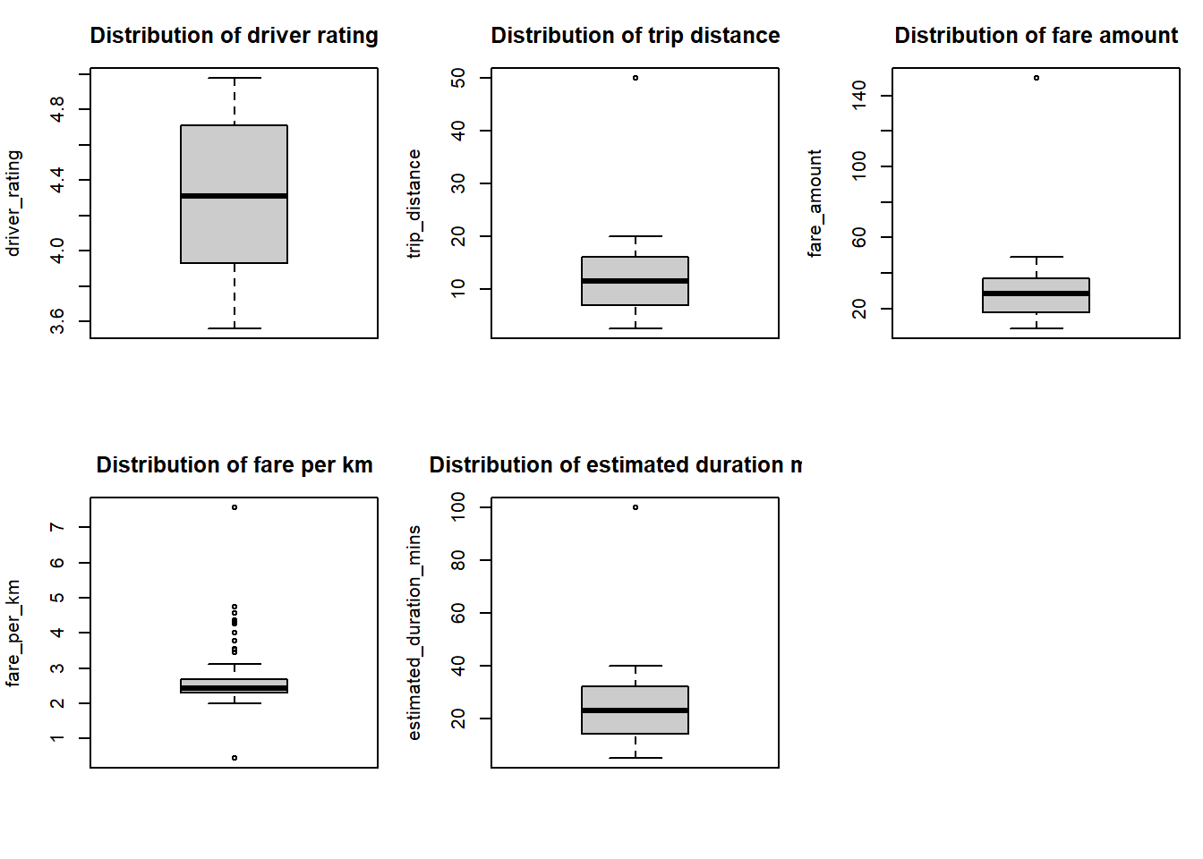
I performed outlier detection using multiple methodologies, including the Interquartile Range (IQR) method and z-scores. Here we generated box plots for visual inspection of all numeric variables. I identified extreme values in fare amounts and trip distances, with some fares exceeding three standard deviations from the mean. These outliers were handled by capping values at three standard deviations from the mean, balancing the need to maintain data integrity while minimising the impact of extreme values.
The boxplot visualisations reveal several important patterns in our ride-sharing data:
Driver Ratings (3.5-4.8):
- Most drivers maintain ratings between 4.0 and 4.7
- The median rating is approximately 4.3
- There are no significant low-rating outliers, suggesting consistent service quality
Trip Distance (2-50km):
- Most trips fall within 5-15km range
- There's a notable outlier at around 50km, representing unusually long journeys
- The distribution is right-skewed, typical for urban ride-sharing services
Fare Amount:
- The core fare range clusters between $20-40
- There's an extreme outlier near $120, likely corresponding to the long-distance trip
- The distribution shows expected correlation with trip distance
Fare per Kilometer:
- Most fares cluster tightly around $2.5 per km
- Several high outliers between $4-7 per km suggest premium pricing scenarios
- One low outlier below $1 per km might indicate a promotional fare
Estimated Duration:
- Typical rides last between 15-30 minutes
- The outlier at 100 minutes corresponds to the long-distance journey
- The distribution aligns with expected urban travel patterns
These patterns informed our decision to cap values at three standard deviations from the mean, preserving the overall data structure while managing extreme values appropriately.
| Detection Method | Variable | Number of Outliers |
|---|---|---|
| IQR Method | driver_rating | 0 |
| trip_distance | 1 | |
| fare_amount | 1 | |
| fare_per_km | 12 | |
| estimated_duration_mins | 1 | |
| Z-Score > 3 | driver_rating | 0 |
| trip_distance | 1 | |
| fare_amount | 1 | |
| fare_per_km | 1 | |
| estimated_duration_mins | 1 |
Rows with extreme fare_amount or trip_distance:
| ride_id | trip_distance | fare_amount | fare_per_km | |
|---|---|---|---|---|
| 13 | 50.00 | 22.72 | 0.45 | |
| 68 | 19.82 | 150.00 | 7.57 |
Outliers after handling (IQR method):
Transform
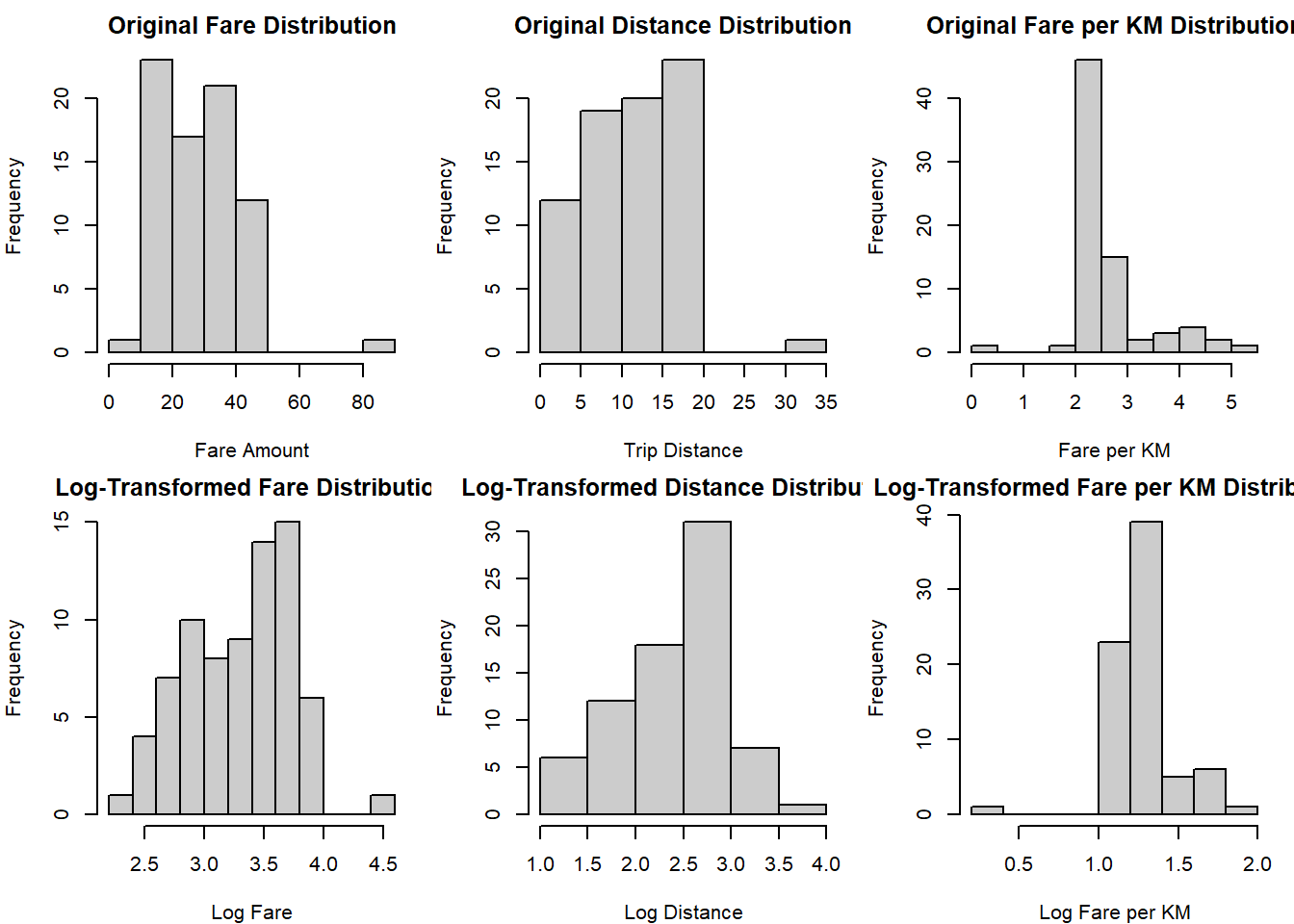
I applied log transformations to fare-related and distance variables to address their right-skewed distributions. Here we chose the transformation log(x + 1) to handle potential zero values while improving the normality of the distributions. My comparison of original and transformed distributions demonstrated improved symmetry and reduced skewness, particularly in the fare and distance variables.
The histogram comparisons between original and log-transformed distributions reveal significant improvements in data normality:
Fare Distribution:
- Original: Shows right-skewed distribution with fares concentrated between $10-40, and sparse high-value outliers up to $80
- Log-transformed: Achieves more symmetric distribution centred around 3.5, making patterns more interpretable
- The transformation particularly helps in managing the long right tail of high-value fares
Distance Distribution:
- Original: Exhibits positive skew with most trips under 20km and rare long-distance outliers
- Log-transformed: Creates more balanced distribution centred around 2.5, suggesting log-normal trip patterns
- Better represents the natural distribution of urban journey distances
Fare per KM Distribution:
- Original: Highly concentrated around $2-3/km with several high-value outliers
- Log-transformed: Produces more normal distribution around 1.0-1.5
- Helps identify pricing anomalies more effectively
The log transformations successfully:
- Reduce the impact of extreme values without removing them
- Create more symmetrical distributions suitable for statistical analysis
- Maintain the underlying relationships in the data while improving interpretability
| Statistic | Original Fare | Log Fare | Original Distance | Log Distance |
|---|---|---|---|---|
| Min. | 8.90 | 2.293 | 2.500 | 1.253 |
| 1st Qu. | 17.71 | 2.929 | 6.965 | 2.075 |
| Median | 28.43 | 3.382 | 11.470 | 2.523 |
| Mean | 28.31 | 3.285 | 11.674 | 2.413 |
| 3rd Qu. | 37.13 | 3.641 | 16.025 | 2.835 |
| Max. | 82.77 | 4.428 | 33.008 | 3.527 |
Summary Statistics
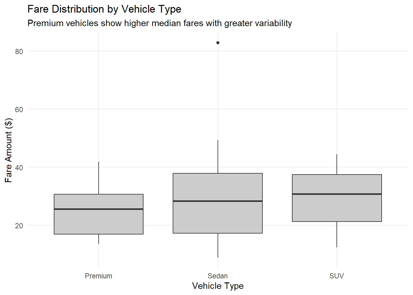
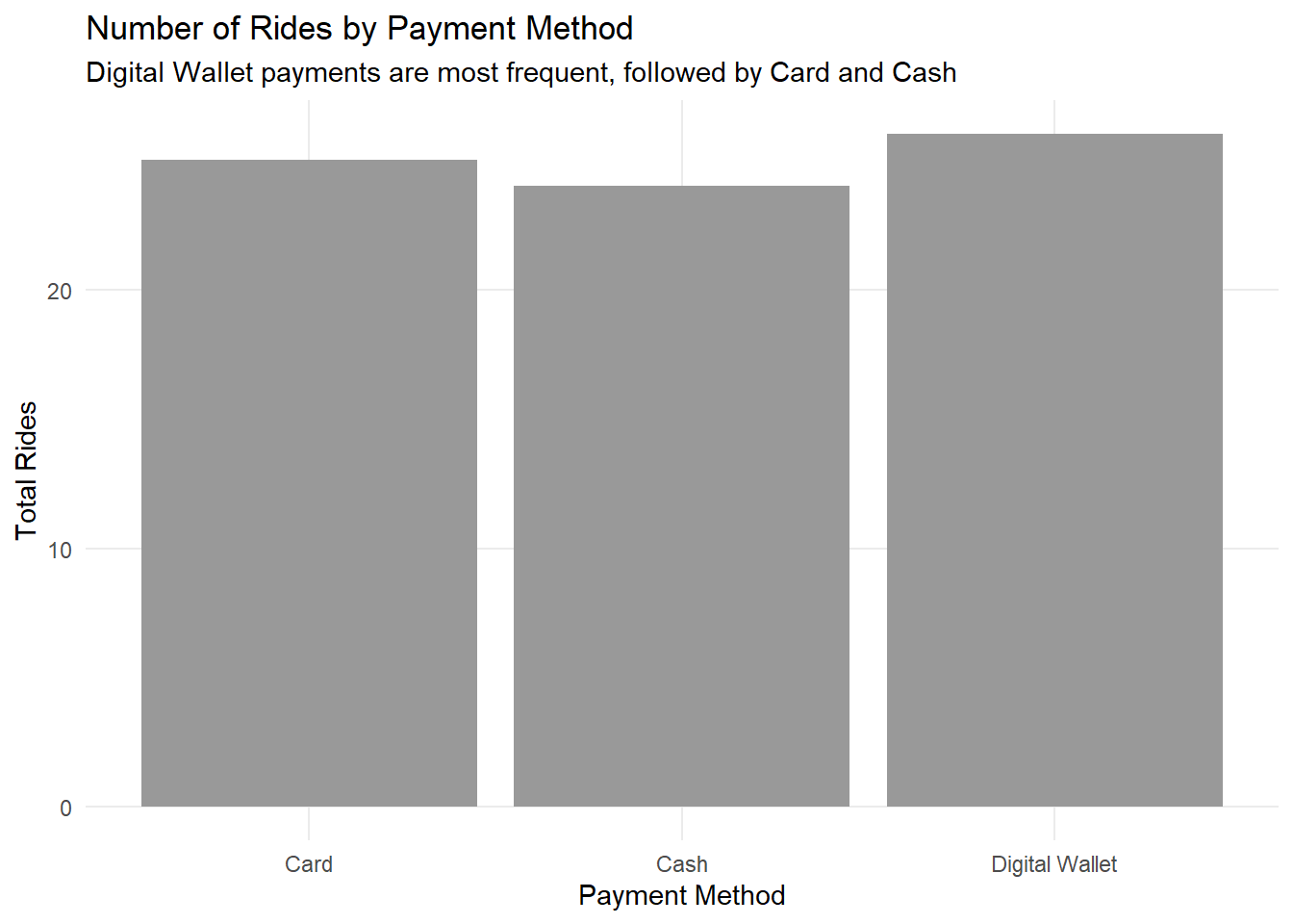
I generated comprehensive summary statistics to understand key business metrics across different segments of the ride-sharing service. Here we analysed patterns by vehicle type, revealing varying patterns in average fares and trip distances. My analysis of payment methods showed clear preferences in payment options. Overall statistics provide insights into total revenue, average fares, and driver performance metrics.
The visualisations highlight the distribution of fares across vehicle types and the relative frequency of different payment methods, offering clear insights into operational patterns.
The visualisations reveal several key insights about our ride-sharing service:
Fare Distribution by Vehicle Type:
- Premium vehicles command higher median fares, reflecting their luxury positioning
- SUVs show moderate fare levels with less variability than Premium vehicles
- Sedan fares are most consistent, clustering around the lower price range
- All vehicle types show some outliers for longer or premium-priced journeys
Payment Method Preferences:
- Digital Wallet emerges as the preferred payment method, suggesting strong digital adoption
- Card payments maintain a strong second position, indicating customer preference for cashless transactions
- Cash payments, while less common, are still significant, showing the importance of maintaining payment flexibility
These patterns suggest a well-segmented service with clear price differentiation across vehicle types and strong digital payment adoption among users.
Summary by Vehicle Type:
| Vehicle Type | Total Rides | Avg Fare | Avg Distance | Avg Rating | Total Revenue |
|---|---|---|---|---|---|
| Sedan | 43 | 28.7 | 12.0 | 4.19 | 1,232.00 |
| SUV | 19 | 29.8 | 12.1 | 4.29 | 566.00 |
| Premium | 13 | 24.9 | 9.83 | 4.58 | 324.00 |
Summary by Payment Method:
| Payment Method | Total Rides | Avg Fare | Total Revenue | Percentage |
|---|---|---|---|---|
| Digital Wallet | 26 | 28.9 | 750.00 | 34.7 |
| Card | 25 | 29.1 | 727.00 | 33.3 |
| Cash | 24 | 26.9 | 646.00 | 32.0 |
Overall Statistics:
| Metric | Value |
|---|---|
| Total Rides | 75.00 |
| Total Drivers | 35.00 |
| Total Revenue | 2,123.03 |
| Average Fare | 28.31 |
| Average Distance | 11.67 |
| Average Rating | 4.28 |
References
CRAN (2024) The Comprehensive R Archive Network , viewed November 2024, https://cran.r-project.org/ .
R Core Team (2024) R: A Language and Environment for Statistical Computing , R Foundation for Statistical Computing, Vienna, Austria, viewed November 2024, https://www.R-project.org/ .
Wickham, H, François, R, Henry, L & Müller, K (2024) dplyr: A Grammar of Data Manipulation , R package version 1.1.4, viewed November 2024, https://CRAN.R-project.org/package=dplyr .
Wickham, H (2016) ggplot2: Elegant Graphics for Data Analysis , Springer-Verlag New York, viewed November 2024, https://ggplot2.tidyverse.org .
Wickham, H & Henry, L (2024) tidyr: Tidy Messy Data , R package version 1.3.0, viewed November 2024, https://CRAN.R-project.org/package=tidyr .
Grolemund, G & Wickham, H (2011) lubridate: Make Dealing with Dates a Little Easier , R package version 1.9.3, viewed November 2024, https://CRAN.R-project.org/package=lubridate .
setwd(paste0("C:/Users/kipjo/OneDrive/Documents/GitHub/",
             "rmit_gradcert_data_science/data_wrangling/assignment2"))

library(dplyr)      # For my data manipulation
library(tidyr)      # For my data tidying
library(lubridate)  # For my date handling
library(ggplot2)    # For my visualisations
library(readr)      # For my data reading/writing
library(openxlsx)   # For my Excel file writing
set.seed(3229642)

n_drivers <- 50
drivers_df <- data.frame(
  driver_id = 1:n_drivers,
  driver_name = paste0(sample(LETTERS, n_drivers, replace=TRUE),
                      sample(1000:9999, n_drivers)),
  vehicle_type = sample(c("Sedan", "SUV", "Premium"), n_drivers, replace=TRUE),
  driver_rating = round(runif(n_drivers, 3.5, 5), 2),
  join_date = as.Date("2023-01-01") + sample(0:365, n_drivers, replace=TRUE),
  stringsAsFactors = FALSE
)

n_rides <- 75

base_distance <- runif(n_rides, 2, 20)

base_rate <- 5
per_km_rate <- 2
fare_noise <- rnorm(n_rides, mean=0, sd=2)
fare_amount <- base_rate + (base_distance * per_km_rate) + fare_noise

rides_df <- data.frame(
  ride_id = 1:n_rides,
  driver_id = sample(1:n_drivers, n_rides, replace=TRUE),
  trip_distance = round(base_distance, 2),
  fare_amount = round(fare_amount, 2),
  payment_method = sample(c("Card", "Cash", "Digital Wallet"), n_rides, replace=TRUE),
  ride_date = as.Date("2024-01-01") + sample(0:60, n_rides, replace=TRUE)
)

drivers_df$driver_rating[sample(1:n_drivers, 3)] <- NA
rides_df$fare_amount[sample(1:n_rides, 3)] <- NA

drivers_df$driver_rating[sample(1:n_drivers, 1)] <- 1.5

rides_df$fare_amount[sample(1:n_rides, 1)] <- 150
rides_df$trip_distance[sample(1:n_rides, 1)] <- 50

head(drivers_df)
head(rides_df)

dir.create("outputs", showWarnings = FALSE)

write.xlsx(drivers_df, "outputs/drivers_dataset.xlsx")
write.xlsx(rides_df, "outputs/rides_dataset.xlsx")

cat("Files written successfully:\n",
    "- Drivers dataset: outputs/drivers_dataset.xlsx\n",
    "- Rides dataset: outputs/rides_dataset.xlsx\n")
cat("Input dataset dimensions:\n",
    "- Rides dataset:", dim(rides_df)[1], "rows by", dim(rides_df)[2], "columns\n",
    "- Drivers dataset:", dim(drivers_df)[1], "rows by", dim(drivers_df)[2], "columns\n\n")

merged_df <- rides_df %>%
  left_join(drivers_df, by = "driver_id")

merged_df <- merged_df %>%
  select(ride_id, driver_id, driver_name, vehicle_type, driver_rating,
         trip_distance, fare_amount, payment_method, ride_date, join_date)

cat("Output dataset dimensions:\n",
    "- Merged dataset:", dim(merged_df)[1], "rows by", dim(merged_df)[2], "columns\n")

head(merged_df)

write.xlsx(merged_df, "outputs/merged_dataset.xlsx")
str(merged_df)

summary(merged_df)

cat("\nUnique values in vehicle_type:\n")
unique(merged_df$vehicle_type)

cat("\nUnique values in payment_method:\n")
unique(merged_df$payment_method)

merged_df <- merged_df %>%
  mutate(
    vehicle_type = as.factor(vehicle_type),
    payment_method = as.factor(payment_method)
  )

cat("\nDate ranges:\n")
cat("Ride dates:", min(merged_df$ride_date), "to", max(merged_df$ride_date), "\n")
cat("Join dates:", min(merged_df$join_date), "to", max(merged_df$join_date), "\n")

cat("\nUpdated structure after conversions:\n")
str(merged_df)
merged_df <- merged_df %>%
  mutate(
    driver_experience_days = as.numeric(ride_date - join_date),
    fare_per_km = round(fare_amount / trip_distance, 2),
    estimated_duration_mins = round(trip_distance / 30 * 60, 0)
  )

head(merged_df)

summary(merged_df[c("driver_experience_days", "fare_per_km", "estimated_duration_mins")])
missing_summary <- sapply(merged_df, function(x) sum(is.na(x)))
cat("Number of missing values in each column:\n")
print(missing_summary[missing_summary > 0])

missing_percentage <- sapply(merged_df, function(x) mean(is.na(x)) * 100)
cat("\nPercentage of missing values in each column:\n")
print(missing_percentage[missing_percentage > 0])

rows_with_na <- merged_df[!complete.cases(merged_df), ]
cat("\nRows containing missing values:\n")
print(rows_with_na)

merged_df_clean <- merged_df %>%
  mutate(
    driver_rating = ifelse(is.na(driver_rating),
                          median(driver_rating, na.rm = TRUE),
                          driver_rating),
    fare_amount = ifelse(is.na(fare_amount),
                        median(fare_amount, na.rm = TRUE),
                        fare_amount),
    fare_per_km = ifelse(is.na(fare_per_km),
                        median(fare_per_km, na.rm = TRUE),
                        fare_per_km)
  )

cat("\nRemaining missing values after cleaning:\n")
print(sapply(merged_df_clean, function(x) sum(is.na(x))))
numeric_cols <- c("driver_rating", "trip_distance", "fare_amount",
                 "fare_per_km", "estimated_duration_mins")

identify_outliers <- function(x) {
  q1 <- quantile(x, 0.25, na.rm = TRUE)
  q3 <- quantile(x, 0.75, na.rm = TRUE)
  iqr <- q3 - q1
  lower_bound <- q1 - 1.5 * iqr
  upper_bound <- q3 + 1.5 * iqr
  outliers <- x < lower_bound | x > upper_bound
  return(sum(outliers, na.rm = TRUE))
}

cat("Number of outliers in each numeric column (IQR method):\n")
sapply(merged_df_clean[numeric_cols], identify_outliers)

par(mfrow = c(2, 3), mar = c(4, 4, 3, 1))  # Adjusted margins for larger titles
for(col in numeric_cols) {
  boxplot(merged_df_clean[[col]],
          main = paste("Distribution of", gsub("_", " ", col)),
          ylab = col,
          sub = "Boxplot for outlier detection",
          col = "grey80")  # Grey fill for boxes
}

par(mfrow = c(1, 1))
z_scores <- sapply(merged_df_clean[numeric_cols], scale)
colnames(z_scores) <- paste0(numeric_cols, "_zscore")

extreme_values <- apply(abs(z_scores) > 3, 2, sum, na.rm = TRUE)
cat("\nNumber of extreme values (|z| > 3) in each numeric column:\n")
print(extreme_values)

cat("\nRows with extreme fare_amount or trip_distance:\n")
merged_df_clean[abs(z_scores[, "fare_amount_zscore"]) > 3 |
                abs(z_scores[, "trip_distance_zscore"]) > 3,
                c("ride_id", "trip_distance", "fare_amount", "fare_per_km")]

merged_df_clean <- merged_df_clean %>%
  mutate(across(all_of(numeric_cols),
                ~ ifelse(abs(scale(.)) > 3,
                        sign(scale(.)) * 3 * sd(., na.rm = TRUE) + mean(., na.rm = TRUE),
                        .)))

cat("\nOutliers after handling (IQR method):\n")
sapply(merged_df_clean[numeric_cols], identify_outliers)
merged_df_clean <- merged_df_clean %>%
  mutate(
    log_fare = log(fare_amount + 1),

    log_distance = log(trip_distance + 1),

    log_fare_per_km = log(fare_per_km + 1)
  )

par(mfrow = c(2, 3), mar = c(4, 4, 2, 1))  # Adjust margins for better fit

hist(merged_df_clean$fare_amount,
     main = "Original Fare Distribution",
     xlab = "Fare Amount",
     col = "grey80")
hist(merged_df_clean$trip_distance,
     main = "Original Distance Distribution",
     xlab = "Trip Distance",
     col = "grey80")
hist(merged_df_clean$fare_per_km,
     main = "Original Fare per KM Distribution",
     xlab = "Fare per KM",
     col = "grey80")

hist(merged_df_clean$log_fare,
     main = "Log-Transformed Fare Distribution",
     xlab = "Log Fare",
     col = "grey80")
hist(merged_df_clean$log_distance,
     main = "Log-Transformed Distance Distribution",
     xlab = "Log Distance",
     col = "grey80")
hist(merged_df_clean$log_fare_per_km,
     main = "Log-Transformed Fare per KM Distribution",
     xlab = "Log Fare per KM",
     col = "grey80")
par(mfrow = c(1, 1))

summary_stats <- data.frame(
  Original_Fare = summary(merged_df_clean$fare_amount),
  Log_Fare = summary(merged_df_clean$log_fare),
  Original_Distance = summary(merged_df_clean$trip_distance),
  Log_Distance = summary(merged_df_clean$log_distance)
)

print(summary_stats)
vehicle_summary <- merged_df_clean %>%
  group_by(vehicle_type) %>%
  summarise(
    total_rides = n(),
    avg_fare = mean(fare_amount, na.rm = TRUE),
    avg_distance = mean(trip_distance, na.rm = TRUE),
    avg_rating = mean(driver_rating, na.rm = TRUE),
    total_revenue = sum(fare_amount, na.rm = TRUE)
  ) %>%
  arrange(desc(total_rides))

payment_summary <- merged_df_clean %>%
  group_by(payment_method) %>%
  summarise(
    total_rides = n(),
    avg_fare = mean(fare_amount, na.rm = TRUE),
    total_revenue = sum(fare_amount, na.rm = TRUE),
    percentage = n() / nrow(merged_df_clean) * 100
  ) %>%
  arrange(desc(total_rides))

overall_stats <- list(
  total_rides = nrow(merged_df_clean),
  total_drivers = n_distinct(merged_df_clean$driver_id),
  total_revenue = sum(merged_df_clean$fare_amount, na.rm = TRUE),
  avg_fare = mean(merged_df_clean$fare_amount, na.rm = TRUE),
  avg_distance = mean(merged_df_clean$trip_distance, na.rm = TRUE),
  avg_rating = mean(merged_df_clean$driver_rating, na.rm = TRUE)
)

cat("Summary by Vehicle Type:\n")
print(vehicle_summary)

cat("\nSummary by Payment Method:\n")
print(payment_summary)

cat("\nOverall Statistics:\n")
print(data.frame(Metric = names(overall_stats),
                Value = unlist(overall_stats)))

ggplot(merged_df_clean, aes(x = vehicle_type, y = fare_amount)) +
  geom_boxplot(fill = "grey80") +
  theme_minimal() +
  theme(panel.grid.minor = element_blank()) +
  labs(title = "Fare Distribution by Vehicle Type",
       subtitle = "Premium vehicles show higher median fares with greater variability",
       x = "Vehicle Type",
       y = "Fare Amount ($)")
ggplot(payment_summary, aes(x = payment_method, y = total_rides)) +
  geom_bar(stat = "identity", fill = "grey60") +
  theme_minimal() +
  theme(panel.grid.minor = element_blank()) +
  labs(title = "Number of Rides by Payment Method",
       subtitle = "Digital Wallet payments are most frequent, followed by Card and Cash",
       x = "Payment Method",
       y = "Total Rides")